Neural networks are important! They diagnose illnesses, help you find photos of your cat, decide whether to give you a loan¹. They make up a huge part of what we call “machine learning” or “artificial intelligence,” especially the new, exciting, scary parts of it. And, given the magnitude of the problems they can handle, they’re simpler than you’d expect.

Most explanations of neural networks for lay people are kind of lousy, because they always start by talking about brains. They’ll define neural networks as “computer systems modeled on the human brain” or “programs that learn the same way as people” or even as “artificial brains.” This makes neural networks sound really cool and sexy and also like they might become sentient and destroy us at any moment. But it doesn’t give you any intuition for what they actually do, because neural networks aren’t really modeled on brains. They’re loosely inspired by brains, the same way Hollywood movies are “inspired by true events.” I really dislike the comparison to brains, because it creates a completely unnecessary air of mystery around a system that’s basically just a lot of math. So I wanted to write an introduction to neural networks that demystifies them a bit.

This blog post explains what a neural network is, in a way that assumes no math background and contains no brain metaphors. Without all the math, it won’t be a very complete or very precise explanation, but I hope it will still give you a decent sense of what neural networks do. At each step, I’ll fill in some of the math-y details in a separate section; feel free to read it or skip it.

Defining the Task

In a typical machine learning task, you’re trying to find a mathematical formula, or model, that takes in some information and uses it to answer a specific question. For example, you might train a model to:

In this context, the machine isn’t learning to speak or play chess or play the violin, it’s just “learning” a formula that you plug numbers into and get numbers out of. The hard part, of course, is figuring out exactly what formula to use - this is called training the model. This blog post focuses on supervised machine learning, where we train the model by feeding it a bunch of examples that have already been labelled with the correct answer. (You can also use neural networks for unsupervised learning, which uses unlabelled data, but that’s beyond the scope of this blog post.)

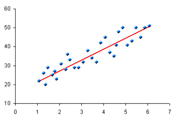
You can think of training a model as trying to come up with the best formula to predict something. You can also think of it as finding the line of best fit for your data:

Random data points on a graph and their line of best fit.

Training the Model

One common technique for training a supervised learning model is an algorithm called gradient descent. Here’s the gist of it:

Get some sample data that includes both the input and the answer you want for the question you care about.
Make an initial guess about what formula to use.
Run your formula on all your training data to get a bunch of predicted answers.
Calculate how close your predicted answers were to the real answers - the error.
Make some tiny adjustments to your formula to reduce the error a bit.
Repeat steps 3-5 until the error is pretty small.

Say you’re throwing a dinner party and you need to know how much wine to buy. You could just consult Emily Post, but instead, you decide to use MACHINE LEARNING. Let’s go through the steps above:

You need training data. So you call three friends who just threw really great dinner parties, and you ask them how many people they invited and how much wine they bought.

Number of Guests	Bottles of wine consumed
3	2
10	7
75	50

You assume that on average, each person will drink about the same amount of wine, so you can model how much to buy with the following formula:
\[\textrm{Number of bottles} = A \times \textrm{Number of guests}\]
Our goal is to find the best value of A. You make an initial guess of one bottle of wine per person, so you set A=1, which gives you:
\[\textrm{Number of bottles} = 1 \times \textrm{Number of guests}\]

For each dinner party in your dataset, you use your formula to calculate how much wine to buy:

Number of guests	Predicted bottles of wine
3	3
10	10
75	75

Now compare your prediction to the correct answers from your training set, and see how close you were:

Number of guests	Predicted bottles of wine	Actual bottles of wine	Error
3	3	2	1
10	10	7	3
75	75	50	25

This formula overestimated how much wine you need, so you reduce A to 0.8. The new formula is: $\textrm{Number of bottles} = 0.8 \times \textrm{Number of guests}$

You try again with your new formula:

Number of guests	Predicted bottles of wine	Actual bottles of wine	Error
3	2.4	2	0.4
10	8	7	1
75	60	50	10

That’s better, but you’re still overestimating how much wine to buy, so you reduce A a bit more. As you get closer and closer to the right value for A, you’ll make smaller and smaller adjustments, so you don’t overshoot the best answer. You’ll continue this process until you have a pretty good model, which in this case will be around A=0.67. Then you can figure out how much wine you need and throw a fabulous party. 🍷

In this example we sort of eyeballed how to adjust A. Real machine learning programs will automatically calculate the error and adjust the model parameters, repeating this process hundreds or thousands of times.

Math-y Details

In a more realistic problem, you would also want a constant term in the model: $y = ax + b$ Most machine learning problems use more than one input (e.g. to predict housing prices you’d look at square feet and number of bedrooms and zip code and so on). So you can generalize this to:

\[y = a_1x_1 + a_2x_2 + \cdots + a_nx_n + b\]

Each $x_i$ here is called an input feature.

In step 4) we calculated the error for each data point, but you actually need to measure how well the model does overall, across the whole data set. You can measure this using the mean squared error, or L2 loss.

Some notation: if there are $m$ data points in the training set, I’ll write the correct answer for the $i^{\textrm{th}}$ data point as $y^i$. (The i there isn’t an exponent - I’m using a superscript to label different data points because I’m using subscripts to label different input features for the same data point.) I’ll use $ŷ^i$ to notate the answer the model predicts for the ith data point. So the equation for the overall error (also called the cost function) will be:

\[\textrm{Err} = \frac{1}{2m}\sum_{i=1}^{m} (y^i - ŷ^i)^2\]

E.g. with the data from step 4:

\[\begin{align} \textrm{Err} & = ((2 - 3)^2 + (7 - 10)^2 + (50 - 75)^2) / (2 \cdot 3) \\\\ & = 105.83 \end{align}\]

Step 5 is updating each parameter in a way that will reduce this error. In the simplest case, where there’s just one input (e.g. number of guests) and just one parameter $a$, you can use this formula to adjust that parameter (where the left arrow means we’re assigning a new value to a):

\[a \leftarrow a - \lambda\frac{d}{da}\textrm{Err}\]

($\lambda$ is the learning rate - it controls how large an adjustment to make at each step. Unlike the other values here, which are calculated automatically, you have to choose $\lambda$ yourself.)

To understand why this works, imagine plotting the error for different values of parameter $a$: Hand-drawn, sort of parabola-shaped graph where x-axis is a (the parameter) and y-axis is error. Minimum of the graph is labelled "best value of a." You’re looking for the value of $a$ that makes the error smallest - the minimum of this graph. At the minimum, the slope of the graph will be 0, so $\frac{d}{da}\textrm{Err}$. If $a$ is too small, this derivative will be negative, so the formula above will increase it. If $a$ is too big, the derivative will be positive, so the formula will decrease $a$. The further away $a$ is from the minimum, the steeper the slope, so the larger the adjustment to $a$.

Note that this process will only find a local minimum, not necessarily a global minimum.

Hand-drawn, squiggly graph where x-axis is a (the parameter) and y-axis is error. There are multiple local minima, labelled with confused question marks

But this particular error function will only have one local minimum, so it works out.

To generalize this to multiple parameters, just take the partial derivative of the error with respect to each of those parameters:

\[a_i \leftarrow a_i - \lambda\frac{\partial}{\partial a_i}\textrm{Err}\]

Neural Networks vs. Other Models

The example above used a linear model: for every extra person you invite, the amount of wine you need goes up by a fixed amount. Depending on the parameters you find during gradient descent, your linear model might look like any of these²:

Scatterplot with line of best fit with years on x-axis and seconds on y-axis. The line trends downward.

Another scatterplot with line of best fit, trending slowly upward

Scatterplot with line of best fit with very steep positive slope.

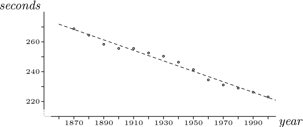
But no matter what parameters you use, it will always be a straight line.

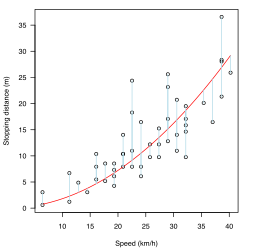
But a linear equation might not always fit your data well. The best model for your data might be quadratic:

Plot of speed vs stopping distance with a quadratic fit

Or logarithmic³:

Graph of logarithm

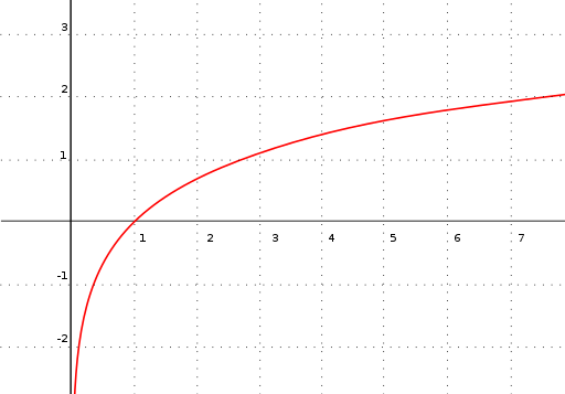
…or something else entirely. The point is, this approach works well if you can choose an appropriate model, one that’s basically the correct shape. But to choose an appropriate model, you already need to understand how your inputs relate to the correct answer. You can sort of eyeball this on a graph if you have one input, but not if you have a hundred.

Let’s go back to the dinner party example. Maybe you didn’t get nice linear data - maybe you can’t see any correlation between the size of a party and how much wine was consumed. So you call your friends back and ask them about their parties. It turns out that a lot of factors go into dinner party planning. Of course, some people drink and others don’t. But there are other complications. Your Aunt Agatha glares disapprovingly at drinkers; if she is invited, everyone will stick to ginger ale. Your Aunt Dahlia is the life of the party; if she’s invited, everyone will have more than usual. (The question of why your aunts are invited to your friends’ dinner parties is beyond the scope of this blog post.) Last year, two of your friends had a nasty divorce and everyone took sides; if people from both factions come to the party, at least one faction will leave in a huff before you’ve served the appetizers. And that’s just the tip of the iceberg - there may be dozens or hundreds of similar factors at play that you don’t even know about.

This is the sort of problem neural networks are good at. They’re flexible enough to fit any relationship between your inputs and output, so you don’t need to understand how they relate ahead of time. And they can figure out how different combinations of inputs will impact your output. A particular guest at your dinner party will have different impacts on different groups of people - a neural network can suss out the different rules for all these different interactions.

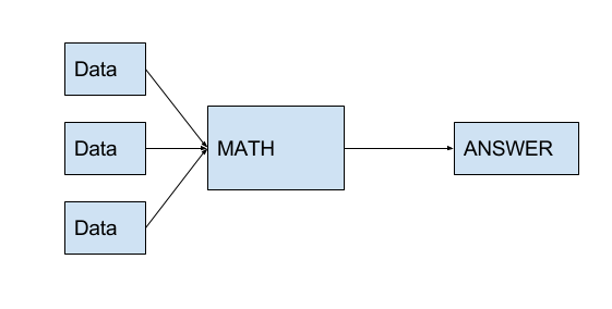
The math behind them isn’t complicated - it’s just function composition, calling functions on the outputs of other functions. So, where the example above looked like this:

$$ \textrm{Answer} = \textrm{MATH}(x_1, x_2, \cdots, x_n) $$

Diagram with three boxes labelled DATA leading to a box labelled MATH leading to a box labelled ANSWER

Then a neural net is just this:

$$ \textrm{Answer} = \textrm{MATH}(\textrm{MATH}(x_1, x_2, \cdots, x_n) + \textrm{MATH}(x_1, x_2, \cdots, x_n) + \cdots) $$

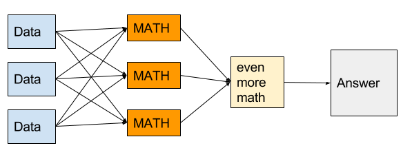
Diagram with three boxes labelled DATA on the left, three boxes labelled MATH in the middle, another box labelled "even more math" to the right, and a box labelled ANSWER furthest right. Each DATA box leads to all three MATH boxes, each MATH box leads into the "even more math" box which leads into the answer

Each of the “math” boxes above is called a neuron. The idea is that each neuron in the first layer (the orange column in the figure) will calculate some relevant information, like “are people from Friend Group A and Friend Group B present?” directly from the inputs you give it. Each bit of relevant information is a feature. Then the neuron in the last layer uses all these features to calculate the answer you really care about. You don’t know in advance what features are important; the neural network will figure them out when you train it.

Neural networks work because individual neurons can capture information about the interactions between inputs, instead of trying to understand each input in isolation. In many machine learning problems, you can’t learn a whole lot from looking at one input at a time; you have to consider how your different inputs interact. At your dinner party, the presence or absence of a single guest can only tell you so much; the social dynamics between guests dictate how much wine they drink. Or think of a photograph: you can’t learn anything from the color of a single pixel. You have to look at the contrast between pixels to make out edges, shapes, and objects.

Let’s build a neural network for our dinner party example. Suppose you have three people you could invite to a dinner party: your aunts Agatha and Dahlia, and your best friend Stiffy. Since just the number of guests doesn’t give you enough information, you need to use the whole guest list as an input. Let’s represent it as a list of numbers, where each position in the list represents one possible guest, in this order:

[Agatha Dahlia Stiffy]

A zero means the friend is not at the party, and a one means they are at the party. So if only Agatha is coming, the list will be:

[1 0 0]

And if Dahlia and Stiffy are coming, it will be:

[0 1 1]

Now you need to figure out what the first layer of neurons should calculate. You’ll need a function called ReLU (short for rectified linear unit), which is almost identical to the linear function from the earlier example, except it flattens out at zero if its input is ever negative:

\[\textrm{ReLU}(n) = \bigg\{ \begin{align} & n \textrm{ if } n > 0 \\ & 0 \textrm{ if } n \leq 0 \end{align}\]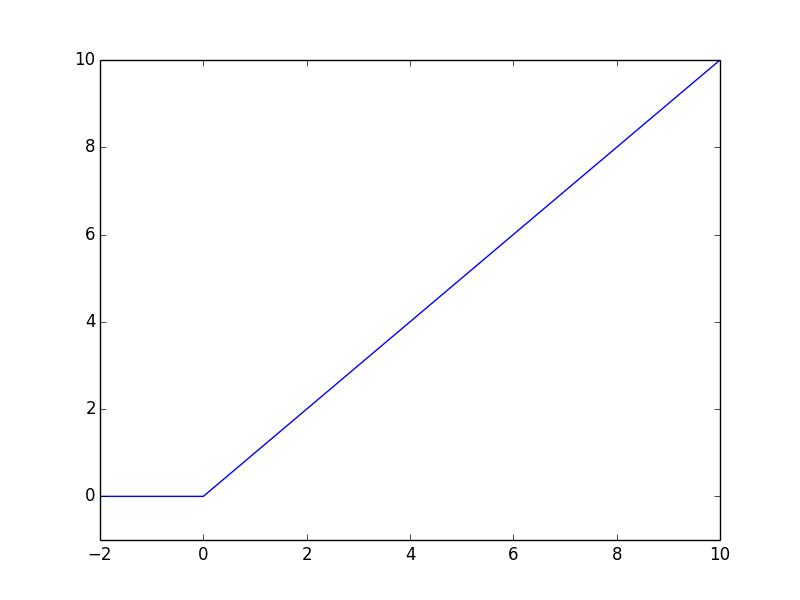

Graph of ReLU function

Here’s a slightly more precise version of the neural network diagram above:

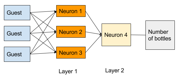
Diagram with three boxes labelled Guest on the left, three orange boxes labelled Neuron 1, Neuron 2, and Neuron 3 in the middle, another box labelled "Neuron 4" to the right, and a box labelled Number of bottles furthest right. Each DATA box leads to each of neuron 1, neuron 2, and neuron 3, and each of these leads into "neuron 4" box which leads to the "bottles of wine" box

Based on this diagram, you have two layers in your neural network. The orange boxes make up layer one. We’ll label the outputs of the three neurons in this layer $\textrm{neuron}_1$, $\textrm{neuron}_2$, and $\textrm{neuron}_3$. Each neuron will have its own set of parameters $a_i$, $b_i$, $c_i$, and $d_i$. You’ll need to figure out the values of these parameters when you train the model. Then each neuron will calculate:

\[\textrm{neuron}_i = \textrm{ReLU}(a_i \times \textrm{Agatha} + b_i \times \textrm{Dahlia} + c_i \times \textrm{Stiffy} + d_i)\]

So, for example, if only Stiffy is coming to your party, $\textrm{neuron}_2$ would calculate:

\[\begin{align} \textrm{neuron}_2 & = \textrm{ReLU}(a_2 \times \textrm{Agatha} + b_2 \times \textrm{Dahlia} + c_2 \times \textrm{Stiffy} + d_2) \\\\ & = \textrm{ReLU}(a_2 \times 0 + b_2 \times 0 + c_2 \times 1 + d_2) \\\\ & = \textrm{ReLU}(c_2 + d_2) \end{align}\]

The second layer of the network has only one neuron - $\textrm{neuron}_4$ in the diagram above. This neuron will have three more parameters $w$, $x$, $y$, and $z$, which you’ll also need to find by training the model. It will calculate:

\[\textrm{Number of bottles} = \textrm{ReLU}(w \times \textrm{neuron}_1 + x \times \textrm{neuron}_2 + y \times \textrm{neuron}_3 + z)\]

If you put it all together, the formula will be:

\[\begin{align} \textrm{Number of bottles} = \textrm{ReLU}( & w \times\textrm{ReLU}(a_1 \times \textrm{Agatha} + b_1 \times \textrm{Dahlia} + c_1 \times \textrm{Stiffy} + d_1) + \\\\ & x \times\textrm{ReLU}(a_2 \times \textrm{Agatha} + b_2 \times \textrm{Dahlia} + c_2 \times \textrm{Stiffy} + d_2) + \\\\ & y \times\textrm{ReLU}(a_3 \times \textrm{Agatha} + b_3 \times \textrm{Dahlia} + c_3 \times \textrm{Stiffy} + d_3) + \\\\ & z) \end{align}\]

Now, just like in the last section, you need to figure out your parameters: $a_1$, $b_2$, $x$, $y$, $z$, and so on. It turns out that you can use exactly the same system as when you were just looking at number of guests; the only difference is that you’ll first do the “tiny adjustments” step for the last layer, then work your way backwards to first layer. This system of making corrections one layer at a time is called backpropagation of errors.

So the new training process is:

Convince your friends to give you the guest lists for all their parties.
Choose random values for every parameter to create an initial model.
Run all the guest lists through the model.
See whether the model over- or under-estimated how much wine was needed for each guest list.
Adjust $w$, $x$, $y$, and $z$ by a little to reduce the error. This means you need to figure out whether each individual neuron tends to overestimate or underestimate. For example, if the model tends to overestimate when the first neuron spits out a big value, you need to make $w$ a bit smaller; but if you mostly overestimate when the second neuron is big, then you need to decrease $x$ more than $w$.
Adjust $a_1$, $b_1$, …, $c_3$, $d_3$ by a little to reduce the error. You can re-use the information from step 5 about when individual neurons over- or under-estimate. You might find that $\textrm{neuron}_1$ tends to overestimate when Agatha is invited to a party, but underestimate when Dahlia is invited; then you’d want to decrease $a_1$ and increase $b_1$. That will help correct $\textrm{neuron}_1$, which will make the final answer a little more accurate.
Repeat steps 3 - 6 until the error is pretty small. Like in the last example, your program will automatically run the model, calculate the error, and adjust all the parameters hundreds or thousands of times.

When you’re finally done training the model, you might end up with something close to this:

\[\begin{align} \textrm{Number of bottles} = \textrm{ReLU}( & 0.5 \times\textrm{ReLU}(0 \times \textrm{Agatha} + 0 \times \textrm{Dahlia} + 1 \times \textrm{Stiffy}) + \\\\ & 2 \times\textrm{ReLU}(0 \times \textrm{Agatha} + 1.5 \times \textrm{Dahlia} + 0.4 \times \textrm{Stiffy} + - 0.5) + \\\\ & -5 \times\textrm{ReLU}(1 \times \textrm{Agatha} + 0 \times \textrm{Dahlia} + 0 \times \textrm{Stiffy}) + \\\\ & 1) \end{align}\]

In this model, each neuron encodes something about people’s drinking habits:

Neuron 1 mean that, left to her own devices, Stiffy will have about half a bottle of wine.
Neuron 2 means that when Dahlia is around, she’ll have a couple bottles, and Stiffy will have more than usual.
Neuron 3 means that when Agatha is present, nobody drinks anything.
And that $+ 1$ at the end, our $z$ value, means that if nobody shows up you’ll have a bottle of wine by yourself.

And that, more or less, is how neural networks can help you plan a dinner party.

Math-y Details

The cost function here will be the same as in the earlier, simpler example:

\[\textrm{Err} = \frac{1}{2}\sum_{i=1}^{m} (y^i - ŷ^i)^2\]

The formula for updating each parameter is the same too:

\[\textrm{param}_i \leftarrow \textrm{param}_i - \lambda\frac{\partial}{\partial \textrm{param}_i}\textrm{Err}\]

Updating the layer 2 parameters (w, x, y, and z) looks exactly the same as in the earlier example. Updating the layer 1 parameters ($a_i$, $b_i$, $c_i$) is more complicated - you need to use the chain rule to calculate the partial derivatives:

\[\begin{align} & \textrm{param}_i \leftarrow \textrm{param}_i - \lambda\frac{\partial}{\partial \textrm{param}_i}\textrm{Err} \\\\ & \textrm{param}_i \leftarrow \textrm{param}_i - \lambda\frac{\partial}{\partial \textrm{param}_i}\textrm{neuron}_i \times \frac{\partial}{\partial \textrm{neuron}_i}\textrm{Err} \end{align}\]

There’s one wrinkle here - because our formula for calculating $ŷ^i$ has gotten more complicated, the cost function is not guaranteed to have only one local minimum - i.e. it’s not convex. That means gradient descent won’t necessarily find the best solution, but it still finds a pretty good one, most of the time.

If you notice any mistakes in this blog post, please email me! This post mostly rehashes the Coursera course on neural networks and deep learning, so if you enjoyed this post you might want to take the course.

In an earlier version of this post, the error in the “Math-y Details” section was calculated incorrectly. Thanks to KGruel for the correction!

¹ Medical diagnosis, Photo recognition, Credit scores. ↩

² Attributions: left graph by Nicholas Longo (Derived from imaged in work by Jim Hefferon) [CC BY-SA 2.5 (https://creativecommons.org/licenses/by-sa/2.5)], via Wikimedia Commons. Middle graph by Jsmura - Own work, CC BY-SA 4.0, https://commons.wikimedia.org/w/index.php?curid=34406311. Right graph by Krishnavedaladerivative work: Cdang - This file was derived fromLinear least squares example2.svg:, CC BY-SA 3.0, https://commons.wikimedia.org/w/index.php?curid=25430567 ↩

³ Graph by Adrian Neumann (Own work) [GFDL (http://www.gnu.org/copyleft/fdl.html), CC-BY-SA-3.0 (http://creativecommons.org/licenses/by-sa/3.0/) or CC BY-SA 2.5-2.0-1.0 (https://creativecommons.org/licenses/by-sa/2.5-2.0-1.0)], via Wikimedia Commons ↩